Claude Model Launches vs NVIDIA H100 Rental Prices
Data-driven analysis exploring how Claude model launches correlate with NVIDIA H100 rental price spikes, revealing timing-sensitive effects across Hyperscaler, Marketplace, and Neocloud providers.

The generative AI arms race has reshaped demand for high-end GPUs like NVIDIA’s H100, but measuring why prices move has remained elusive. This report tackles a key hypothesis: do major foundation model releases—specifically Anthropic’s Claude models—drive immediate market reactions in H100 rental pricing?
Using real-world price indices and historical event alignment, we analyze H100 cost fluctuations across different provider types (Hyperscaler, Marketplace, and Neocloud) to identify patterns that correlate with Claude release dates. The goal: to quantify cause-and-effect where speculation usually dominates.
Our findings show measurable pricing impact around Claude milestones—and reveal how each segment of the cloud GPU market responds differently to new model pressure.
TL;DR
- There are measurable, but source-type-specific, signals between Claude launch timing and H100 rental price movements.
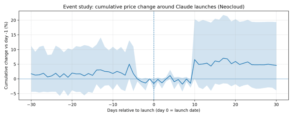
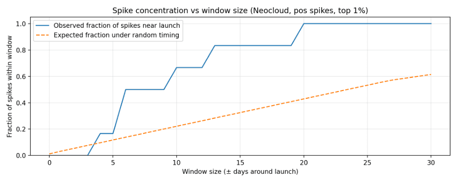
- The clearest signal is in Neocloud pricing: top 1% positive price jumps cluster within about a 2-week window around launches (5 of 6 spikes within ±14 days; hypergeometric enrichment p=0.011).
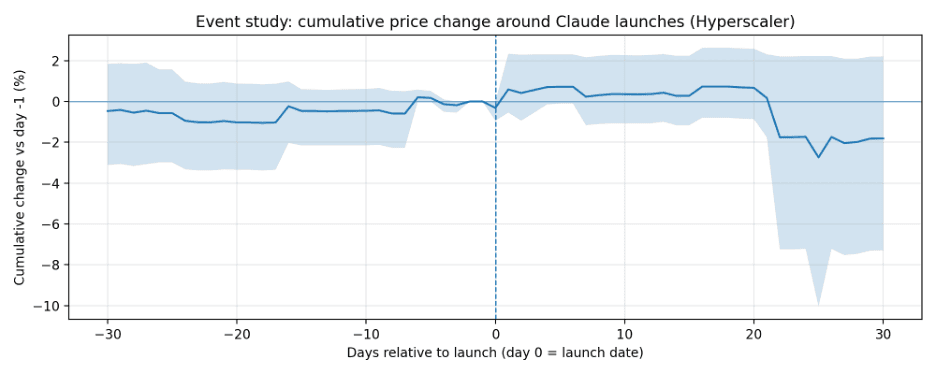
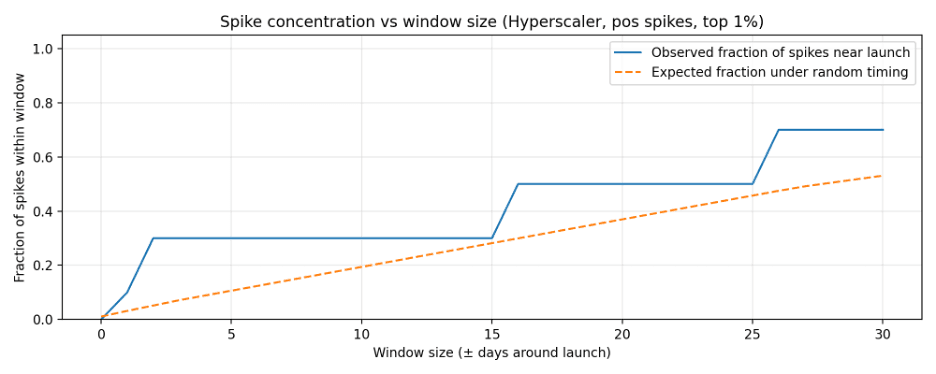
- Hyperscaler pricing shows short-horizon concentration: 3 of the top 10 positive jumps occur within ±3 days of a launch (p=0.029). Direction is mixed: the average same-day move is slightly negative, but there is often a rebound within a few days.
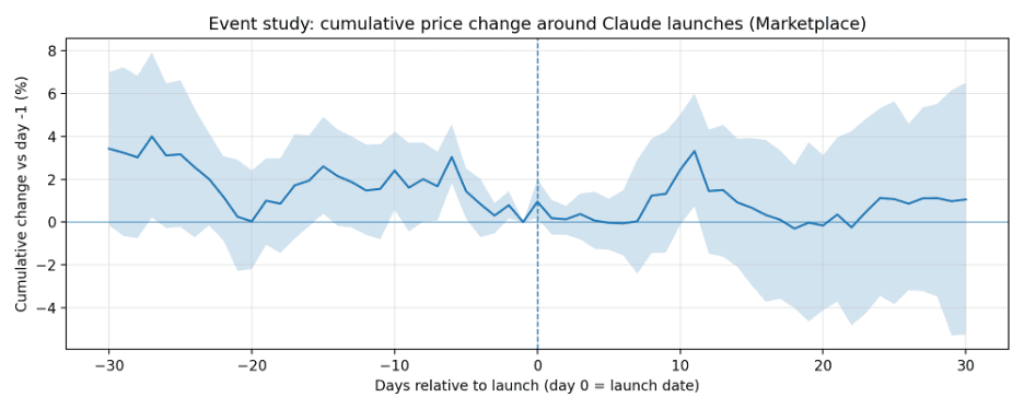
- Marketplace pricing shows no statistically meaningful spike concentration around launches in this dataset.
- These patterns are correlations (not causality) and are based on a small number of launch events and relatively coarse price sampling for some source types.
Claude launch calendar
| Date | Launches | # launches |
|---|---|---|
| 2024-02-29 | Claude 3 Opus | 1 |
| 2024-03-07 | Claude 3 Haiku | 1 |
| 2024-06-20 | Claude 3.5 Sonnet (20240620) | 1 |
| 2024-10-22 | Claude 3.5 Haiku, Claude 3.5 Sonnet (20241022) | 2 |
| 2025-02-19 | Claude 3.7 Sonnet | 1 |
| 2025-05-14 | Claude Opus 4, Claude Sonnet 4 | 2 |
| 2025-08-05 | Claude Opus 4.1 | 1 |
| 2025-09-29 | Claude Sonnet 4.5 | 1 |
| 2025-10-01 | Claude Haiku 4.5 | 1 |
| 2025-11-24 | Claude Opus 4.5 | 1 |
H100 price data coverage (raw)
| Source | Obs | Days | Start | End | Min | Max | Mean |
|---|---|---|---|---|---|---|---|
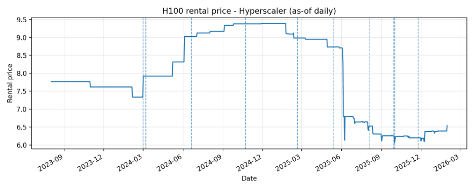
| Hyperscaler | 913 | 913 | 2023-08-02 | 2026-01-30 | 6.06 | 9.387 | 7.956 |
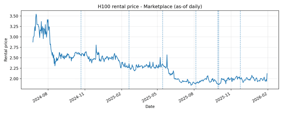
| Marketplace | 586 | 586 | 2024-06-24 | 2026-01-30 | 1.838 | 3.546 | 2.293 |
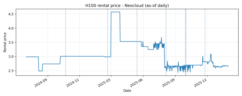
| Neocloud | 507 | 507 | 2024-07-01 | 2026-01-30 | 2.436 | 4.572 | 3.069 |
Note: Marketplace and Neocloud series begin in mid-2024. Launches before the first observed quote for a given source_type are excluded from that source's event-window statistics.
Methodology
- Daily time series construction: For each source_type, prices are reindexed to a daily calendar and forward-filled ("as-of" series). No backfilling is applied before the first observed quote to avoid creating artificial pre-history.
- Return definition: Daily log-return r_t = log(P_t) - log(P_{t-1}). A "positive spike" is a day in the top 1% of r_t for that source_type.
- Event windows: A launch day is day 0. We examine windows of ±30 days for visualization and shorter windows (±3, ±7, ±14) for spike concentration tests.
- Event study (price level): For each launch day d, compute cumulative log change log(P_{d+k}) - log(P_{d-1}) for k in [-30, +30]. Average across launches; bootstrap across events to form 95% confidence intervals.
- Spike enrichment test: Compare the observed number of top-1% spike days that fall within ±k days of a launch versus the expected number under random timing. A hypergeometric enrichment p-value is reported.
- Volatility near launches: Compute the mean absolute return |r_t| on days within ±7 days of launches and compare to a random baseline using a permutation (Monte Carlo) test.
Results
Price series with Claude launch markers
Dashed vertical lines indicate Claude launch days included for each source_type.
Hyperscaler
Marketplace
Neocloud
Event study: average cumulative price change around launches
Cumulative change is measured versus day -1. Shaded regions are 95% bootstrap confidence intervals.
Hyperscaler
Marketplace
Neocloud
Positive spike concentration around launches
Definition: positive spike = top 1% daily log-return for that source_type. The enrichment p-value tests whether the observed number of spikes near launches is higher than expected under random timing.
Positive spike enrichment (top 1% daily returns)
| Source | Window (±days) | # spikes | # near | Expected share | Observed share | p (enrich) |
|---|---|---|---|---|---|---|
| Hyperscaler | 3 | 10 | 3 | 0.071 | 0.3 | 0.0289 |
| Hyperscaler | 7 | 10 | 3 | 0.141 | 0.3 | 0.1571 |
| Hyperscaler | 14 | 10 | 3 | 0.264 | 0.3 | 0.5174 |
| Marketplace | 3 | 6 | 0 | 0.075 | 0.0 | 1.0000 |
| Marketplace | 7 | 6 | 1 | 0.157 | 0.167 | 0.6435 |
| Marketplace | 14 | 6 | 2 | 0.301 | 0.333 | 0.5826 |
| Neocloud | 3 | 6 | 0 | 0.076 | 0.0 | 1.0000 |
| Neocloud | 7 | 6 | 3 | 0.159 | 0.5 | 0.0543 |
| Neocloud | 14 | 6 | 5 | 0.304 | 0.833 | 0.0113 |
Volatility near launches
Permutation p-value tests whether mean |return| is higher on near-launch days (±7) than under random timing.
Near-launch volatility test (±7 days)
| Source | Window (±days) | Near days | Total days | Mean |r| (near) | Mean |r| (null) | p (greater) |
|---|---|---|---|---|---|---|
| Hyperscaler | 7 | 129 | 912 | 0.0019 | 0.0014 | 0.2296 |
| Marketplace | 7 | 92 | 585 | 0.0112 | 0.0151 | 0.9900 |
| Neocloud | 7 | 92 | 578 | 0.0203 | 0.0112 | 0.0123 |
Notable Neocloud spike instances
Top 1% positive Neocloud return days, mapped to the nearest Claude launch:
| Spike date | Approx. +% | Nearest launch | Lag (days) | Launch |
|---|---|---|---|---|
| 2025-03-01 | 52.9 | 2025-02-19 | 10 | Claude 3.7 Sonnet |
| 2025-09-09 | 15.6 | 2025-09-29 | -20 | Claude Sonnet 4.5 |
| 2025-09-25 | 10.1 | 2025-09-29 | -4 | Claude Sonnet 4.5 |
| 2025-10-07 | 10.2 | 2025-10-01 | 6 | Claude Haiku 4.5 |
| 2025-10-14 | 10.1 | 2025-10-01 | 13 | Claude Haiku 4.5 |
| 2025-11-18 | 11.8 | 2025-11-24 | -6 | Claude Opus 4.5 |
Spike-window concentration curves (Neocloud and Hyperscaler):
Permutation tests on event-day and short-horizon moves
These tests compare launch-day metrics to randomly sampled dates (excluding ±30 days around launches). Max |cum. move| (0..7) is the maximum absolute cumulative move within days 0..7 relative to day -1.
| Source | Metric | Actual mean | Null mean | p (two-sided) | p (>) | p (<) | # events |
|---|---|---|---|---|---|---|---|
| Hyperscaler | Return on day 0 | -0.0032 | 0.0001 | 0.0256 | 0.9989 | 0.0012 | 10 |
| Hyperscaler | Max cum. move (0..7) | 0.0074 | 0.0015 | 0.0198 | 0.0197 | 0.9803 | 10 |
| Hyperscaler | Max |cum. move| (0..7) | 0.0189 | 0.0029 | <0.0001 | <0.0001 | 1.0000 | 10 |
| Marketplace | Return on day 0 | 0.0095 | -0.0006 | 0.3290 | 0.1635 | 0.8366 | 7 |
| Marketplace | Max cum. move (0..7) | 0.026 | 0.0295 | 0.8325 | 0.5504 | 0.4496 | 7 |
| Marketplace | Max |cum. move| (0..7) | 0.0359 | 0.0607 | 0.1474 | 0.9447 | 0.0554 | 7 |
| Neocloud | Return on day 0 | -0.0159 | -0.0012 | 0.0867 | 0.9390 | 0.0611 | 7 |
| Neocloud | Max cum. move (0..7) | 0.0129 | 0.0061 | 0.3692 | 0.2852 | 0.7149 | 7 |
| Neocloud | Max |cum. move| (0..7) | 0.0352 | 0.0234 | 0.6454 | 0.2824 | 0.7176 | 7 |
Interpretation and limitations
- Segment differences matter. Signals are most visible in Neocloud and (to a lesser extent) Hyperscaler; Marketplace appears less responsive in this sample.
- Timing is not purely same-day. For Neocloud, several spike days occur a few days before/after launches, and one very large spike occurs 10 days after the 2025-02-19 launch (Claude 3.7 Sonnet). This is consistent with market adjustments or demand/supply shifts that lag announcements.
- Confounding is likely. H100 pricing is influenced by many factors (supply availability, competitor launches, broader AI demand, outages, contract repricing cadence). This analysis does not isolate causal effects.
- Sample size is small. Marketplace/Neocloud only have 7 usable launch windows, so statistical power is limited and confidence intervals are wide.
Conclusion
- There is evidence of correlation between Claude launch timing and H100 rental price spikes, but it is not uniform across source types.
- Neocloud shows the strongest signal: positive spikes concentrate within ±14 days of launches (p=0.011).
- Hyperscaler shows short-window concentration (±3 days; p=0.029) and elevated short-horizon movement in 0..7 days (permutation p < 0.0001), though direction is mixed.
- Marketplace shows no robust spike concentration signal in this dataset.
Forward-looking next steps
- Add control events: include other frontier model launches (OpenAI, Google, etc.) to test whether the signal is Claude-specific or reflects broader AI demand cycles.
- Use richer market features: incorporate utilization/availability metrics (if accessible) and separate spot vs reserved pricing; spikes in price without volume can be misleading.
- Move from correlation to causal inference: build a synthetic control (or difference-in-differences) using non-launch periods and/or other GPU SKUs as controls.
- Model lead/lag explicitly: regress returns on distributed lags/leads of launch indicators to estimate a response curve and isolate typical delay patterns.