The Illusion of Stability: Unpacking H100 GPU Market Value Trends
The Illusion of Stability: Unpacking H100 GPU Market Value Trends
A 2026 guide to real-world LLM token costs, model pricing, and proven ways to reduce spend
Written by
Yang Gao
Data Analyst at Silicon Data
#
Use Cases
Jan 30, 2026
0 Mins Read
You're reading
The Illusion of Stability: Unpacking H100 GPU Market Value Trends
Table of Content
Data window: June 2024 – December 2025
Model: NVIDIA H100 (Launch: October 2022)
Sources: Global retail and resale listings (NEW, USED, REFURBISHED)
The NVIDIA H100 was never meant to be ordinary. As the world’s most coveted AI accelerator, its performance dominance was matched by a staggering retail price—typically ranging from $25,000 to $40,000 throughout mid-2024 into early 2026. On paper, this looked like unprecedented price stability. No discounting, no market erosion, no fire sales. For over a year, the sticker price of the H100 seemed frozen in time.
But underneath that stable facade, a very different story was unfolding.
In this report, we analyze thousands of H100 retail and resale listings between June 2024 and December 2025, covering multiple geographies and SKU variants. While retail prices remained flat, secondary market data showed steep, sometimes chaotic depreciation—with USED and REFURBISHED H100s trading as high as $50,000 in mid-2024, only to plunge sharply as supply increased and buyer power returned.
This divergence between retail illusion and resale reality reveals critical risks for data center buyers, enterprise procurement teams, and financial planners. Teams that relied on retail pricing as a proxy for asset value found themselves holding inflated book values while the resale market collapsed beneath them.
To fully understand this dynamic, we break depreciation down into two key dimensions:
Time-based depreciation — how price changes relative to age since launch
Market-relative depreciation — how a unit’s value shifts relative to peak and contemporaneous NEW price
Using these buckets, we track early- and mid-life value retention of the H100 across both absolute and relative baselines.
This isn’t just a story about hardware pricing. It’s a wake-up call for how enterprise teams model capex cycles in the new AI infrastructure economy. The H100 doesn’t follow the old rules. It depreciates later—but when it does, the drop is faster, sharper, and often harder to absorb.
How We Analyzed the H100 Depreciation Curve
Methodology Disclaimer
This report describes observed market pricing behavior and derives market value estimates from public retail and resale listings. It is not an accounting depreciation schedule and should not be used for financial reporting, tax, or audit purposes.
Listing prices may differ from executed transaction prices due to negotiation, shipping, taxes, and seller terms.
NEW prices are used as contemporaneous benchmarks only when same-day, same-country, same-model matches exist.
Condition labels (NEW / USED / REFURBISHED) are seller-provided and may contain misclassifications despite filtering.
Results reflect the June 2024–March 2026 observation window shown in this report and may not generalize to later market regimes.
To unpack the real story behind H100 depreciation, we first needed to clean, align, and normalize GPU pricing data from multiple sources. The goal: ensure that price comparisons reflect true asset value, not noise from mismatched models, geographies, or timelines.
Our methodology focused on three major components: data preparation, outlier removal, and model age normalization. Here’s how each step worked:
1. Data Cleaning & Preparation
We began with a global dataset of H100 retail listings collected between June 2024 and December 2025. Each record contained five primary fields:
country
date
condition (NEW / USED / REFURBISHED)
product_slug
retail_price
To ensure consistency, we applied the following normalization steps:
Country normalization: e.g., converting GB to UK
Condition standardization: all labels upper-cased and harmonized
Invalid data removal: excluded any listing with missing or non-positive prices
Deduplication: removed exact duplicates that could distort frequency or average calculations
2. USED–NEW Price Matching Logic
One of the most important aspects of this analysis was ensuring that USED and REFURBISHED prices could be meaningfully compared to their NEW counterparts. To prevent apples-to-oranges comparisons, we required a strict matching logic:
We only retained USED or REFURBISHED listings if a
same-day, same-country, same-model NEW listing
This ensures that observed price ratios reflect true contemporaneous market dynamics, not time-lagged distortions or SKU mismatches.
Retail listing data is messy. Some USED listings show prices above NEW listings due to errors, arbitrage noise, or misclassified conditions. We cleaned this using two filters:
a. Global Ratio Filter
We applied a hard constraint:
0.3≤ used_price / new_price ≤ 1.1
0.3≤ used_price / new_price ≤ 1.1
0.3≤ used_price / new_price ≤ 1.1
0.3≤ used_price / new_price ≤ 1.1
This eliminates clear outliers — for example, listings where USED units were mistakenly priced at 2× their NEW counterparts.
b. Regional IQR Filtering
For more granular filtering, we computed interquartile ranges (IQR) for each (country, condition) group and applied standard statistical bounds:
This strategy keeps the central pricing trend intact while suppressing pricing anomalies. To avoid overfitting, groups with fewer than 8 listings were exempted.
4. Model Age Normalization
To understand depreciation in the context of product lifecycle, we calculated the model age for each listing based on the H100’s official launch date (October 1, 2022):
We lacked true 1-year pricing data, but the dataset provided robust coverage of 2–3 year-old listings, ideal for evaluating the asset’s performance during its most critical TCO window.
How H100 Condition and Asset Age Impact Resale Value
Our depreciation model evaluates H100 resale value by segmenting listings into time-based buckets (2-year and 3-year age) and condition tiers (USED vs. REFURBISHED). The goal: uncover how real-world market behavior values the same hardware at different lifecycle stages.
Key Findings
Refurbished GPUs hold value better across the board.
In the 2-year age window, REFURBISHED H100s typically resell for 80–90% of their contemporaneous NEW price, while USED units average just 65–75%.
Depreciation steepens dramatically in year three.
REFURBISHED units in the 3-year bucket drop further to 70–75%, but USED units fall sharply to just 45–55%, marking a clear mid-life inflection point.
Condition matters more as GPUs age.
The spread between REFURBISHED and USED resale prices widens over time—what starts as a 10–15% gap at year two can grow to a 25–30% delta by year three. That divergence reflects buyer preference for certified or warranty-backed hardware in aging inventory.
This isn’t just cosmetic.
The condition-based premium reflects reduced perceived risk, longer remaining lifespan, and greater compatibility with enterprise procurement standards.
What This Means
In short: H100 resale value depends on both age and condition, but the market does not move linearly. REFURBISHED units stayed in the mid‑80% range versus NEW pricing across 2024–2025, while USED units traded at materially larger discounts and showed higher volatility. Refurbishment acts as a buffer, helping preserve value and broadening market appeal when market conditions shift.
This dynamic is critical for operators, brokers, and finance teams making multi-year hardware bets. If your exit strategy extends beyond the 2‑year mark, refurbishment (or purchasing refurbished) can be one of the most practical ways to reduce downside risk and improve resale predictability.
The Lifecycle of Value: Time-Based Market Value Evolution in H100 GPUs
To assess how the NVIDIA H100 holds value over time, we segmented resale listings into model-age buckets—centered around 2 and 3 years post-launch—anchored to the official October 2022 release date.
This model-age framing allows direct measurement of how the market prices hardware as it matures, independent of product condition alone. And the results are telling.
Used H100s: Discounted and Volatile Repricing
In 2024 (roughly ~2 years post-launch), USED H100s traded at a median of ~61% of the contemporaneous NEW price. By 2025 (~3 years post-launch), the median moved to ~69% — a reminder that secondary-market pricing is often non-linear and can shift with supply waves, listing mix, and buyer expectations, not just hardware age.
Rather than behaving like a smooth “depreciation curve,” the USED segment is best understood as market repricing: values reset quickly as supply loosens, alternative GPUs enter the conversation (e.g., H200 and Blackwell-class systems), and buyers become more selective about risk, warranty, and remaining service life.
Refurbished Units: A Smoother Glide Path
REFURBISHED H100s show a much steadier market value profile. In 2024, refurbished units held around ~85% of contemporaneous NEW pricing, and remained roughly ~84% in 2025. This stability is consistent with what buyers pay for: lower perceived risk, clearer provenance, and (often) stronger warranty or reconditioning assurances.
Condition
2024 (~2-year)
2025 (~3-year)
USED
~61%
~69%
REFURBISHED
~85%
~84%
In practice, refurbishment acts as a value buffer: it narrows downside risk and supports more predictable resale outcomes, especially as the broader market transitions toward newer architectures.
Strategic Implications
The time-based view reinforces a practical takeaway: condition is a first-order driver of market value, and the USED segment can reprice abruptly. Across 2024–2025, refurbished units remained in the mid‑80% range versus NEW pricing, while used units typically cleared at a materially larger discount (low‑60s to high‑60s). For procurement teams, this argues for active exit planning and for treating refurbishment as a lever that can meaningfully stabilize resale outcomes when the market regime shifts.
In short, the H100 age curve is not linear. Timing—and condition—can mean the difference between recovering a mid‑80% resale multiple (refurbished) versus low‑60%–high‑60% outcomes (used), depending on the market regime.
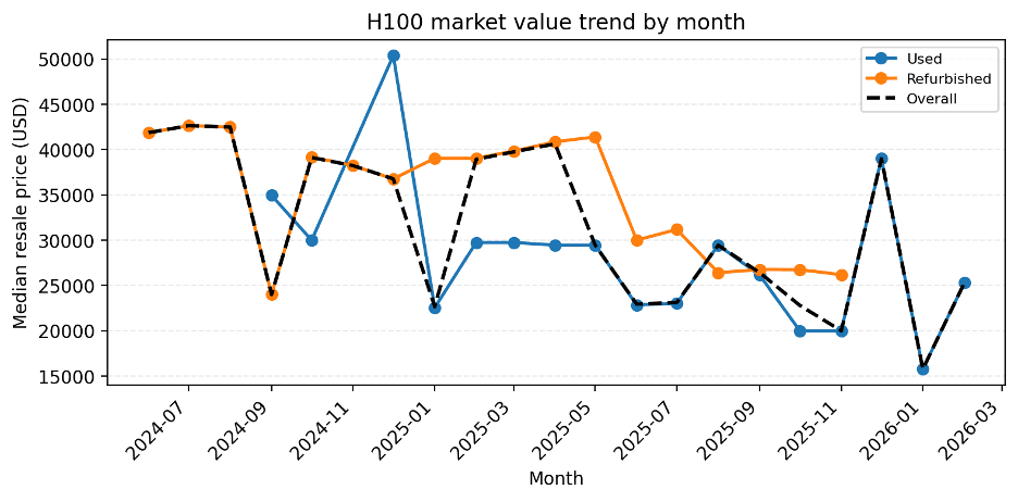
H100 Market Value Trend by Month
Time-based buckets are useful for lifecycle framing, but the secondary market often moves in step-changes. The chart below tracks the median resale listing price by month (USD), split by condition (USED vs. REFURBISHED), with an overall median trend line for context.
What stands out in this monthly view:
A clear downshift from mid‑2024 pricing in the low‑$40Ks toward the mid‑$20Ks by late‑2025, even as primary NEW pricing remained comparatively sticky.
USED pricing is noticeably more volatile than REFURBISHED, with sharp spikes and drops that likely reflect thin monthly supply, listing mix, and episodic demand rather than gradual wear-and-tear effects.
REFURBISHED units typically price above USED units and follow a smoother trajectory, consistent with the premium buyers place on reconditioning and perceived reliability.
Late‑2025 / early‑2026 shows another regime change (a brief rebound followed by a sharp dip), highlighting that market value can reprice quickly when supply conditions or buyer sentiment shifts.
Taken together, this chart reinforces the core framing of this report: H100 value behavior is better described as market-driven repricing and market value estimation, not a smooth depreciation schedule. For planning, the risk is not slow drift — it’s sudden resets.
Peak Price Anchoring: How Much Value H100s Truly Retain
To understand the deeper depreciation trajectory of the NVIDIA H100, we applied an alternative benchmark: comparing resale values not to contemporaneous retail prices, but to each product’s historical peak retail price. This approach reveals how far the asset has fallen from its highest valuation—offering a long-term view that cuts through temporary supply pressures or short-term demand spikes.
Why This Matters
While comparing resale to current retail pricing tells us how used hardware is performing today, peak anchoringanswers a more fundamental question:
“How much value does this GPU still retain relative to when it was worth the most?”
For capital planning and depreciation modeling, this view better captures structural value loss—not just recent market conditions.
What We Found
2-year-old H100s now trade at just 30–40% of their historical maximum NEW price.
3-year-old units fall further, with resale values clustering between 20–30% of their peak.
These numbers show that even GPUs with seemingly high resale prices (e.g., $12K–$16K) have already lost the majority of their peak value if they once commanded $40K+.
Model Age
% of Historical Max NEW
2-Year
~30–40%
3-Year
~20–30%
Implication
This baseline makes one thing clear: the H100’s illusion of price stability—anchored by sticky NEW listing prices—breaks down under long-term scrutiny. True asset value erosion is dramatic, even if headline retail prices suggest otherwise.
For buyers and operators, that means planning exit strategies and depreciation models around peak value loss, not nominal price tags. Waiting too long to offload H100s could mean recovering just a fraction of their former worth.
Key Findings: What the H100 Depreciation Curve Really Tells Us
After analyzing over 18 months of H100 resale data, several critical trends emerged that challenge conventional assumptions about GPU lifecycle value:
1. Unusually Strong Early-Life Value Retention
Compared to the previous generation A100, the H100’s secondary-market pricing has been unusually elevated — but not by accident. Even ~2–3 years post-launch, refurbished units held in the mid‑80% range versus contemporaneous NEW pricing, and the market continued to clear used inventory at meaningful but variable discounts. This behavior was reinforced by three forces: the AI boom’s sustained demand shock, the H100’s performance leap over the A100, and the capital/engineering friction of transitioning data centers to newer platforms. Together, these factors supported higher resale multiples and delayed the kind of steady, predictable value drift many teams assume for infrastructure assets.
2. Refurbished Premium Is Real—and Profitable
Across all time buckets, refurbished H100s consistently sell for 15–25 percentage points more than their used counterparts. This points to clear arbitrage opportunities for resellers and suggests refurbishment programs can meaningfully boost hardware ROI.
3. The Mid-Life Cliff Is Steep
Rather than a smooth glide path, the H100 tends to reprice in step-changes. Around the ~2‑year mark, market value becomes more sensitive to supply waves and to new alternatives entering the market. The monthly trend view shows that medians can swing sharply over short windows — especially for USED inventory — which is why timing and channel strategy matter as much as hardware age.
4. Your Depreciation Baseline Changes the Story
Two pricing baselines tell very different stories:
Contemporaneous NEW pricing emphasizes market tightness and supply-demand dynamics
Historical peak pricing exposes deeper long-term capital loss—showing that most H100s retain just 20–40% of their peak value by year 3
Conclusion: Navigating GPU Investment in a Volatile Market
The global data center GPU market, valued at USD 36.59 billion in 2025, is projected to reach USD 48.39 billion in 2026 and an astonishing USD 1,026.28 billion by 2040, growing at a 24.38% compound annual growth rate (CAGR) during the forecast period from 2026 to 2040. This explosive growth reflects the central role GPUs play in powering modern AI workloads across industries—from cloud providers and enterprises to academic research and startups.
But rapid market growth doesn’t guarantee stable asset value. Our analysis reveals that H100 depreciation accelerates sharply after about two years of service, especially for USED inventory. This dynamic runs counter to historical expectations formed during previous GPU generations like the A100, where depreciation was more gradual and predictable. For the H100, early life might appear resilient, but once the inflection point is reached, the resale market quickly revalues assets as short-cycle capital rather than long-term infrastructure.
At the same time, the condition of the GPU plays a growing role in value retention. REFURBISHED H100s consistently outperform USED H100s by 15–25 percentage points, offering a strategic edge for buyers and resellers alike. The preference for refurbished stock underscores the importance of quality assurance, warranty backing, and market confidence—attributes that translate to real economic value.
Strategic Considerations for GPU Procurement and Depreciation Modeling
Can the H100 experience inform procurement strategies for other GPUs? Not entirely — and certainly not when looking at the A100, which saw faster and more predictable market value decline. The H100 followed a different curve because it entered the market under extraordinary conditions: surging demand for LLMs and extreme supply scarcity. These factors created a temporary illusion of price stability that defied historical norms.
Incorporate condition premiums into TCO models: The difference between refurbished and used pricing can materially affect ROI calculations, capital planning, and resale projections.
Reassess hardware refresh strategies: Annual GPU architecture advances (e.g., H200, Blackwell, and others) compress the useful life of current models and elevate obsolescence risk.
Use data-driven baselines: Benchmark market value using both contemporaneous NEW pricing and historical peak pricing to capture short-term market dynamics and long-term value erosion.
Monitor global pricing disparities: Geographic price variations and local market dynamics offer arbitrage opportunities and can inform smarter sourcing.
Because GPUs are now core to AI infrastructure strategy, they should be treated as financial assets with depreciation risk, not static hardware line items. Retail prices can be deceptively stable, but underlying value is slipping faster than most models assume.
For teams managing capital, operations, or procurement, the key question is no longer whether GPUs depreciate—it’s how much, how fast, and under what conditions. The data shows that without proactive planning, organizations risk overstating asset value, misaligning refresh cycles, and ultimately paying more over the life of a GPU than necessary.